Time Bin Encoding
Time bin encoding is a fundamental concept in quantum optics. This tutorial demonstrates how to simulate time bin encoding using the photon_weave package. The Simulation makes use of beam splitters and phase shifters in a structured setup.
Overview
Time Bin Encoding Setup
- The time bin encoding process involves:
Four Beam Splitters
Two Phase Shifters
A high level diagram is as follows:
 """
     ┍━[PS:a]━┑    ┍━[PS:b]━┑
     │        │    │        │
 ━━━[/]━━━━━━[\]━━[/]━━━━━━[\]━━◽
                            ┃
                           ◽
"""
The goal is to simulate the interaction of photons through these components and measure the outcomes at various points in time.
Function Description
def time_bin_encoding(alpha:float, beta:float) -> List[List[int]]
- Parameters:
alpha (float): Phase Shift for the first arm
beta (float): Phase Shift for the second arm
Returns: * List[List[int]]: Measurement outcomes at three time intervals. Each list contains two integers representing the outcomes at the top and bottom detectors
Implementation Steps
1. Imports
First import all of the needed libraries and objects in the top of the file.
import multiprocessing as mp
from functools import partial
from tqdm import tqdm

import jax.numpy as jnp
import matplotlib.pyplot as plt

from photon_weave.operation import CompositeOperationType, FockOperationType, Operation
from photon_weave.state.composite_envelope import CompositeEnvelope
from photon_weave.state.envelope import Envelope
from photon_weave.photon_weave import Config
2. Define MZI
We create the class, which handles our MZI transformations.
class MZI:
    def __init__(self, phase_shift_angle, name, debug=False):
        self.name=name
        self.debug = debug
        self.debug_probabilities_top = []
        self.debug_probabilities_bot = []
        self.phase_shift = Operation(
            FockOperationType.PhaseShift,
            phi=phase_shift_angle
        )
        self.beam_splitter = Operation(
            CompositeOperationType.NonPolarizingBeamSplitter,
            eta=jnp.pi/4
        )

    def _empty_env(self, name):
        """
        Creates an empty envelope, (For debugging purposes)
        """
        env = Envelope()
        env.uid = f"{self.name}-{name}"
        env.fock.uid = f"{self.name}-{name}"
        env.fock.dimensions = 2
        return env

    def debug_log_probabilities(self, top_env, bot_env):
        prob_top = get_probability(top_env)
        prob_bot = get_probability(bot_env)
        self.debug_probabilities_top.append(prob_top)
        self.debug_probabilities_bot.append(prob_bot)

    def show_debug_plot(self):
        labels = ['After BS1', 'Before BS2 1', 'Before BS2 2']

        x = jnp.arange(len(labels))  # X-axis positions

        fig, axs = plt.subplots(2, 1, sharex=True, figsize=(6, 6))

        # Top bar chart
        axs[0].bar(x, self.debug_probabilities_top, color='blue', alpha=0.7)
        axs[0].set_ylabel('Top Probabilities')
        axs[0].set_title('Top and Bottom Probabilities')

        # Bottom bar chart
        axs[1].bar(x, self.debug_probabilities_bot, color='red', alpha=0.7)
        axs[1].set_ylabel('Bottom Probabilities')
        axs[1].set_xlabel('Time Steps')
        axs[1].set_xticks(x)
        axs[1].set_xticklabels(labels)

        plt.tight_layout()
        plt.show()

    def apply_ps(self, env:Envelope) -> Envelope:
        env.fock.apply_operation(self.phase_shift)
        return env

    def apply_bs(self, env_top: Envelope, env_bot: Envelope) -> list[Envelope]:
        ce = CompositeEnvelope(env_top, env_bot)
        ce.apply_operation(self.beam_splitter, env_top.fock, env_bot.fock)
        return env_top, env_bot

    def process(self, env_t0, env_t1=None):
        """
        We process pulses going through one MZI.
        special case is if there is a second pulse at t1.
        """

        results = []
        env01 = self._empty_env(1)

        """
        We rename the pulses as we go through the mzi, so that we can
        keep track of what is happening with them.

        First Pulse, First BeamSplitter
        -----
        - we send one pulse top and one bottom
        - we also apply the phase shift to the pulse going through the top arm
        """
        env_top_first_pulse, env_bot_first_pulse = self.apply_bs(env_t0, env01)
        env_top_first_pulse = self.apply_ps(env_top_first_pulse)
        self.debug_log_probabilities(env_top_first_pulse, env_bot_first_pulse)

        if env_t1:
            """
            We do the same in case we received another pulse at t2
            we label these pulses as second_pulse
            """
            env02 = self._empty_env(2)
            env_top_second_pulse, env_bot_second_pulse = self.apply_bs(
                env_t1, env02
            )
            env_top_second_pulse = self.apply_ps(env_top_second_pulse)

        """
        First pulse (taking shorter path) will always arrive alone.
        we apply the second beam_splitter and append it to the results
        """
        env10 = self._empty_env(10)
        env_top_first_out, env_bot_first_out = self.apply_bs(
            env10, env_bot_first_pulse
        )

        self.debug_log_probabilities(env_top_first_out, env_bot_first_out)
        results.append(
            {
                "top": env_top_first_out,
                "bot": env_bot_first_out
            }
        )

        if env_t1 is None:
            """
            In case there is no second pulse entering MZI, we can
            just interact the top pulse with a new empty one and
            append the pulses to the results
            """
            # There is no interaction with the second pulse
            env12 = self._empty_env(12)
            env_top_second_out, env_bot_second_out = self.apply_bs(
                env_top_first_pulse, env12
            )
            results.append(
                {
                    "top": env_top_second_out,
                    "bot": env_bot_second_out
                }
            )
            self.debug_log_probabilities(env_top_second_out, env_bot_second_out)
        else:
            """
            In case there is second pulse entering MZI, we have simulate interaction
            between the pulse going the long way from first pulse and the pulse taking
            the short way from the second pulse.
            """
            env_top_second_out, env_bot_second_out = self.apply_bs(
                env_top_first_pulse,
                env_bot_second_pulse
            )
            results.append(
                {
                    "top": env_top_second_out,
                    "bot": env_bot_second_out
                }
            )

            """
            Finally we process the part of the second pulse, which
            took the long way and interacts with the vacuum state
            at the last beam-splitter
            """
            env_top_third_out, env_bot_third_out = self.apply_bs(
                env_top_second_pulse,
                self._empty_env("last")
            )
            results.append(
                {
                    "top":env_top_third_out,
                    "bot":env_bot_third_out
                }
            )
        if self.debug:
            self.show_debug_plot()
        return results

    env1 = Envelope()
    env1.fock.state = 3
    env2 = Envelope()
3. Single run for Time-Bin Encoding
We define single run for Time-Bin Encoding, so that we may run it in a loop to generate the plots.
We also define run_tbe in order to enable parallelization.
def tbe(alpha:float, beta:float, runs:int=1):
    """
    Simulates time bin encoding

    Time Bin encoding makes use of four beam splitters
    and two phase shifters (see diagram below):
        ┍━[PS:a]━┑    ┍━[PS:b]━┑
        │        │    │        │
    ———[/]━━━━━━[\]━━[/]━━━━━━[\]━━◽
                               ┃
                              ◽

    Parameters:
    -----------
    alpha (float): phase shift on the first MZI
    beta (float): phase shift on the second MZI
    runs (int): number of runs for the simulation
    Notes:
    ------
    if runs is equal to 1, then the probabilities are extracted from the state.
    if runs > 1, then the states are actually measured and the average outcome is returned.
    """
    assert runs > 0

    probs_top_0 = []
    probs_bot_0 = []
    probs_top_1 = []
    probs_bot_1 = []
    probs_top_2 = []
    probs_bot_2 = []

    mzi_1 = MZI(alpha, "first", debug=False)
    mzi_2 = MZI(beta, "second")


    for i in range(runs):
        # Set the initial pulses
        env1=Envelope()
        env1.fock.state=1
        env1.fock.dimensions=2


        first_pulse, second_pulse = mzi_1.process(env1)
        first_pulse, second_pulse, third_pulse = mzi_2.process(first_pulse["top"], second_pulse["top"])
        if runs == 1:
            probs_top_0.append(get_probability(first_pulse["top"]))
            probs_bot_0.append(get_probability(first_pulse["bot"]))
            probs_top_1.append(get_probability(second_pulse["top"]))
            probs_bot_1.append(get_probability(second_pulse["bot"]))
            probs_top_2.append(get_probability(third_pulse["top"]))
            probs_bot_2.append(get_probability(third_pulse["bot"]))
        else:
            probs_top_0.append(first_pulse["top"].measure()[first_pulse["top"].fock])
            probs_bot_0.append(first_pulse["bot"].measure()[first_pulse["bot"].fock])

            probs_top_1.append(second_pulse["top"].measure()[second_pulse["top"].fock])
            probs_bot_1.append(second_pulse["bot"].measure()[second_pulse["bot"].fock])

            probs_top_2.append(third_pulse["top"].measure()[third_pulse["top"].fock])
            probs_bot_2.append(third_pulse["bot"].measure()[third_pulse["bot"].fock])


    probs_top_0 = jnp.array(probs_top_0)
    probs_bot_0 = jnp.array(probs_bot_0)
    probs_top_1 = jnp.array(probs_top_1)
    probs_bot_1 = jnp.array(probs_bot_1)
    probs_top_2 = jnp.array(probs_top_2)
    probs_bot_2 = jnp.array(probs_bot_2)


    all_probabilities = [probs_top_0, probs_bot_0, probs_top_1, probs_bot_1, probs_top_2, probs_bot_2]
    all_averages = [jnp.mean(p) for p in all_probabilities]
    return all_averages
    ce = CompositeEnvelope(env1, env2)
    ce.apply_operation(bs, env1.fock, env2.fock)

    ce.apply_operation(ps, env1.fock)

            def run_tbe(alpha:float, beta:float, runs:int):
                            """
                            Top level function to run the tbe
                            used for parallelization
                            """
                            return tbe(float(alpha), float(beta), runs=runs)
4. Define Plotting Logic
We define the plotting logic
def get_probability(env:Envelope):
    state = env.fock.trace_out()
    one=jnp.abs(state[1][0])**2
    return float(one)


def plotting(prob0t=0, prob0b=0, prob1t=0, prob1b=0, prob2t=0, prob2b=0):
    labels = ['t0', 't1', 't2']
    top_probs = [prob0t, prob1t, prob2t]
    bottom_probs = [prob0b, prob1b, prob2b]

    x = jnp.arange(len(labels))  # X-axis positions

    fig, axs = plt.subplots(2, 1, sharex=True, figsize=(6, 6))

    # Top bar chart
    axs[0].bar(x, top_probs, color='blue', alpha=0.7)
    axs[0].set_ylabel('Top Probabilities')
    axs[0].set_title('Top and Bottom Probabilities')

    # Bottom bar chart
    axs[1].bar(x, bottom_probs, color='red', alpha=0.7)
    axs[1].set_ylabel('Bottom Probabilities')
    axs[1].set_xlabel('Time Steps')
    axs[1].set_xticks(x)
    axs[1].set_xticklabels(labels)

    plt.tight_layout()
    plt.show()

    bs = Operation(CompositeOperationType.NonPolarizingBeamSplitter, eta=jnp.pi/4)
    s1 = Operation(FockOperationType.PhaseShift, phi=alpha)
    s2 = Operation(FockOperationType.PhaseShift, phi=beta)
5. Main block
Lastly we tie it all together in the __main__ block, enabling different ways or running the example (parallelization, measuring).
if __name__ == "__main__":
"""
Configuration for the simulation.
If RUNS = 1, only one run will be executed for each alpha
value, but the probabilities will be extracted directly from
the state.
If RUNS > 1, the resulting pulses will be measured and the
average outcome will be returned for each pulse
PARALLEL = True, runs will run in parallel, useful for RUNS>1
and larger number of alpha values
PARALLEL = False, runs will run sequentially, useful for RUNS=1
and lower number of alpha value (depending on the cores available)
NOTES:
When running in parallel the whole jax needs to be loaded in each
process, which takes some time.
BETA = float, fixed beta value in the all simulation runs
alpha_values = linspace, alpha values for which the simulation will
be executed
PLOT_FILE_NAME = the name of the resulting plot
"""
RUNS = 1
PARALLEL = False
BETA = 0
alpha_values = jnp.linspace(0, 2*jnp.pi, 100)
PLOT_FILE_NAME = "plots/time_bin_encoding.png"
if PARALLEL:
ctx = mp.get_context("spawn")
with ctx.Pool(processes=mp.cpu_count()) as pool:
run_tbe_partial = partial(run_tbe, beta=BETA, runs=RUNS)
results = list(tqdm(
pool.imap(run_tbe_partial, alpha_values),
total=len(alpha_values),
desc="Computing probabilities"))
else:
results = []
for alpha in tqdm(alpha_values, desc="Computing probabilities"):
results.append(tbe(float(alpha), float(BETA), runs=RUNS))
# Unpack the results and prepare them for the plotting
(
probabilities_top_0, probabilities_bot_0,
probabilities_top_1, probabilities_bot_1,
probabilities_top_2, probabilities_bot_2
) = zip(*results)
probabilities_all = [
[jnp.array(probabilities_top_0), jnp.array(probabilities_bot_0)],
[jnp.array(probabilities_top_1), jnp.array(probabilities_bot_1)],
[jnp.array(probabilities_top_2), jnp.array(probabilities_bot_2)],
]
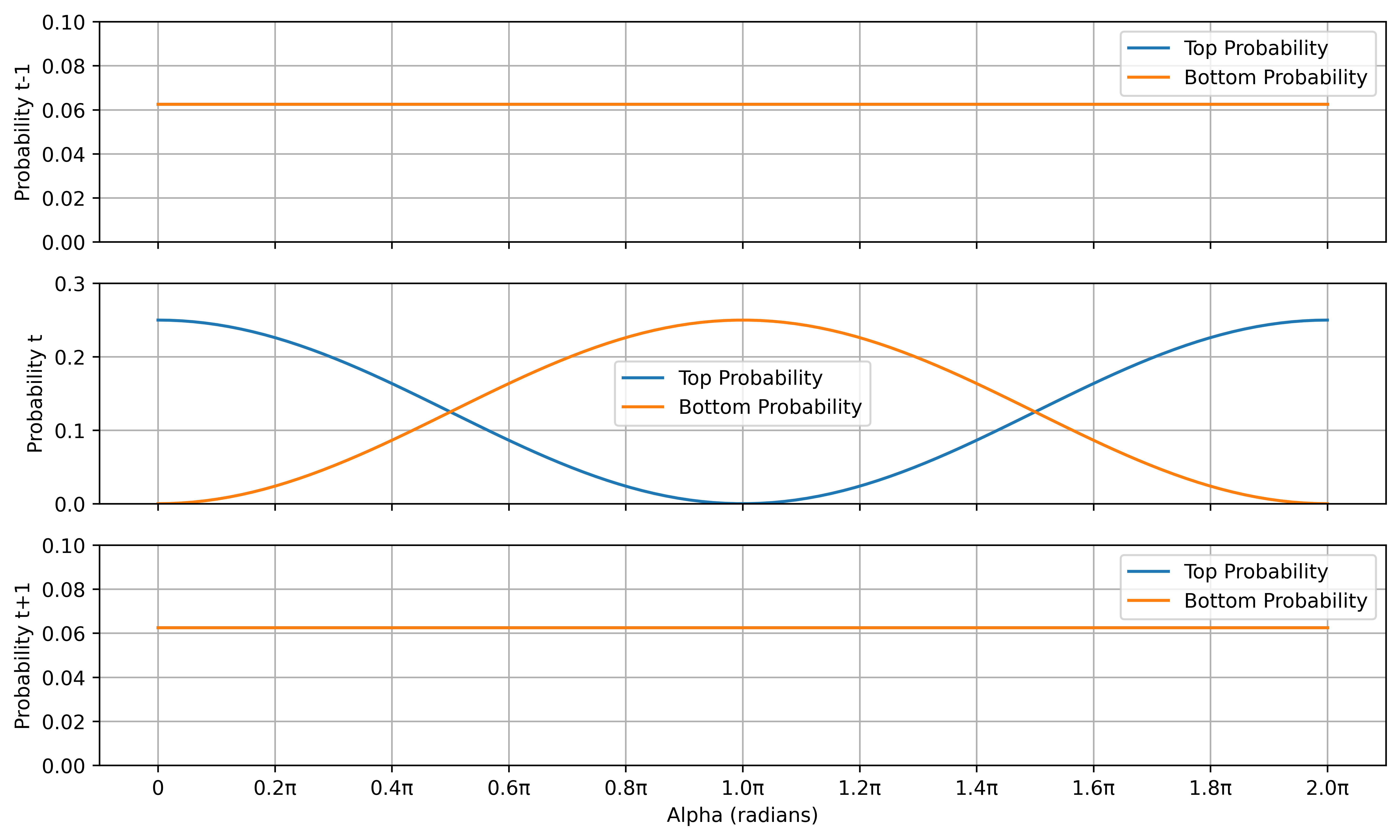
# Plot the probabilities
fig, axes = plt.subplots(3, 1, figsize=(10, 6))
titles = ["t-1", "t", "t+1"]
divisions = 11
xticks = jnp.linspace(0, 2 * jnp.pi, divisions) # 5 divisions from 0 to 2π
xtick_labels = [f"{i:.1f}π" if i > 0 else "0" for i in jnp.linspace(0, 2, divisions)]
ylims = [(0,0.1), (0,0.3), (0,0.1)]
for i, ax in enumerate(axes):
ax.plot(alpha_values, probabilities_all[i][0], label="Top Probability")
ax.plot(alpha_values, probabilities_all[i][1], label="Bottom Probability")
ax.set_ylabel(f"Probability {titles[i]}")
ax.legend()
ax.set_xticks(xticks)
ax.set_xticklabels([])
ax.set_ylim(*ylims[i])
ax.grid(True)
axes[-1].set_xlabel("Alpha (radians)")
axes[-1].set_xticklabels(xtick_labels)
plt.tight_layout()
if PLOT_FILE_NAME:
plt.savefig(PLOT_FILE_NAME, dpi=600, bbox_inches="tight")
else:
plt.show()
tmp_env_0_1 = Envelope()
tmp_env_0_2 = Envelope()
ce = CompositeEnvelope(ce, tmp_env_0_1, tmp_env_0_2)
ce.apply_operation(bs, env2.fock, tmp_env_0_1.fock)
ce.apply_operation(bs, tmp_env_0_2.fock, env1.fock)
Execution
Now we can execute our function, which simulates the time bin encoding.
python time_bin_encoding.py