Jaynes-Cummings Model
The Jaynes-Cummings model is a cornerstone of quantum optics, describing the interaction between a two-level atom (qubit) and a quantized electromagnetic field (mode of a cavity). This tutorial deminstrates how to implement and simulate the Jaynes-Cummings model using the PhotonWeave package.
Implementation
1. Imports
First import all of the needed libraries and objects in the top of the file.
import jax.numpy as jnp
import matplotlib.pyplot as plt
import numpy as np

from photon_weave.state.envelope import Envelope
from photon_weave.state.fock import Fock
from photon_weave.state.composite_envelope import CompositeEnvelope
from photon_weave.state.custom_state import CustomState
from photon_weave.operation import (
    Operation,
    CompositeOperationType,
    FockOperationType
)
from photon_weave.photon_weave import Config
from photon_weave.extra.expression_interpreter import interpreter
2. Interacting States
Create the two states, which will be interacting in the simulation. We represent the light state with the Envelope and the atom state with the CustomState. Since the two systems will be interacting, we put them into one CompositeEnvelope.
env = Envelope()
env.fock.state = 1

qubit = CustomState(2)
qubit.state = 0
ce = CompositeEnvelope(env, qubit)
3. Hamiltonian Construction
Create the parameters, which define the Hamiltonian
h_bar = 1

# System parameters
w_field = 1 * jnp.pi # Angular frequency of the field (radians per second, e.g., 5 GHz)
w_qubit = 1 * jnp.pi  # Angular frequency of the qubit (radians per second, e.g., 5 GHz)
g = 1 * jnp.pi # Coupling strength between the qubit and field (radians per second, e.g., 100 MHz)

# Time parameters
t_delta = 0.01 # Time step for simulation (seconds, e.g., 1 nanosecond)
t_max = 3 # Total simulation time (seconds, e.g., 1 microsecond)
Then we can create the individual parameters which make up the Hamiltonian. The dimensions of the qubit system are fixed, but the simulated dimensions of the Fock systems can change.
# Define the relevant qubit operators
 sigma_z = jnp.array(
     [[1,0],
      [0,-1]])
 sigma_plus = jnp.array(
     [[0,1],
      [0,0]])
 sigma_minus = jnp.array(
     [[0,0],
      [1,0]])

 # Define the relevant Fock operators
 def annihilation_operator(n):
     data = jnp.sqrt(jnp.arange(1, n))
     return jnp.diag(data, k=1)

 def creation_operator(n):
     data = jnp.sqrt(jnp.arange(1, n))
     return jnp.diag(data, k=-1)
Now in order to create our operator based on the Hamiltonian, we need to create a context dictionary, so that PhotonWeave knows how to construct the operator. Dictionary elements must be callable with expecting one parameter: list of dimensions. This is true also for the operators, which operate on the systems with fixed dimensions. Make sure to select the correct dimension element in the callable. The order should reflect the order in which the states are passed to the apply_operation method.
# Define the expression context
context = {
    "a" : lambda dims: annihilation_operator(dims[0]),
    "a_dag" : lambda dims: creation_operator(dims[0]),
    "i_p": lambda dims: jnp.eye(dims[0]),
    "s_z": lambda dims: sigma_z,
    "s_plus": lambda dims: sigma_plus,
    "s_minus": lambda dims: sigma_minus,
    "s_i": lambda dims: jnp.eye(2)
}
With the context defined, we can define our operator based on the well known Hamiltonian. We split the Hamiltonian into three different expressions to keep our sanity. In the last expression (expr) we combine the Hamiltonian and create an operator out of it.
# Field Hamiltonian
H_field = (
    "s_mult",
     h_bar, w_field,
     ("kron",
      ("m_mult",
       "a_dag", "a",),
      "s_i"
     )
)

# Qubit Hamiltonian
H_qubit = (
    "s_mult", h_bar, w_qubit/2,
    ("kron", "i_p", "s_z")
)

# Interaction Hamiltonian
H_interaction = (
    "s_mult", h_bar, g,
    ("add",
     ("kron", "a", "s_plus"),
     ("kron", "a_dag", "s_minus")
     )
    )

# Unitary evolution Hamiltonian
expr = (
    "expm",
    ("s_mult",
        -1j,
        ("add",
             H_field,
             H_qubit,
             H_interaction
             ),
        t_delta,
        1/h_bar
   )
)

# Create the operator with the defined expression
jc_interraction = Operation(
    CompositeOperationType.Expression,
    expr=expr,
    context=context,
    state_types=[
        Fock, CustomState
    ]
)
4. Interacting States
Now we can execute the simulations with capturing the populations after each application of the created unitary operator.
interractions = jnp.arange(0, t_max, t_delta)

qubit_excited_populations = []

for i, step in enumerate(interractions):
    # Apply the operation for the time step
    ce.apply_operation(jc_interraction, env.fock, qubit)

    # Capture the qubit system
    qubit_reduced = qubit.trace_out()
    qubit_reduced = qubit_reduced/jnp.linalg.norm(qubit_reduced)

    # Store the populations
    qubit_excited_populations.append(jnp.abs(qubit_reduced[1][0])**2)
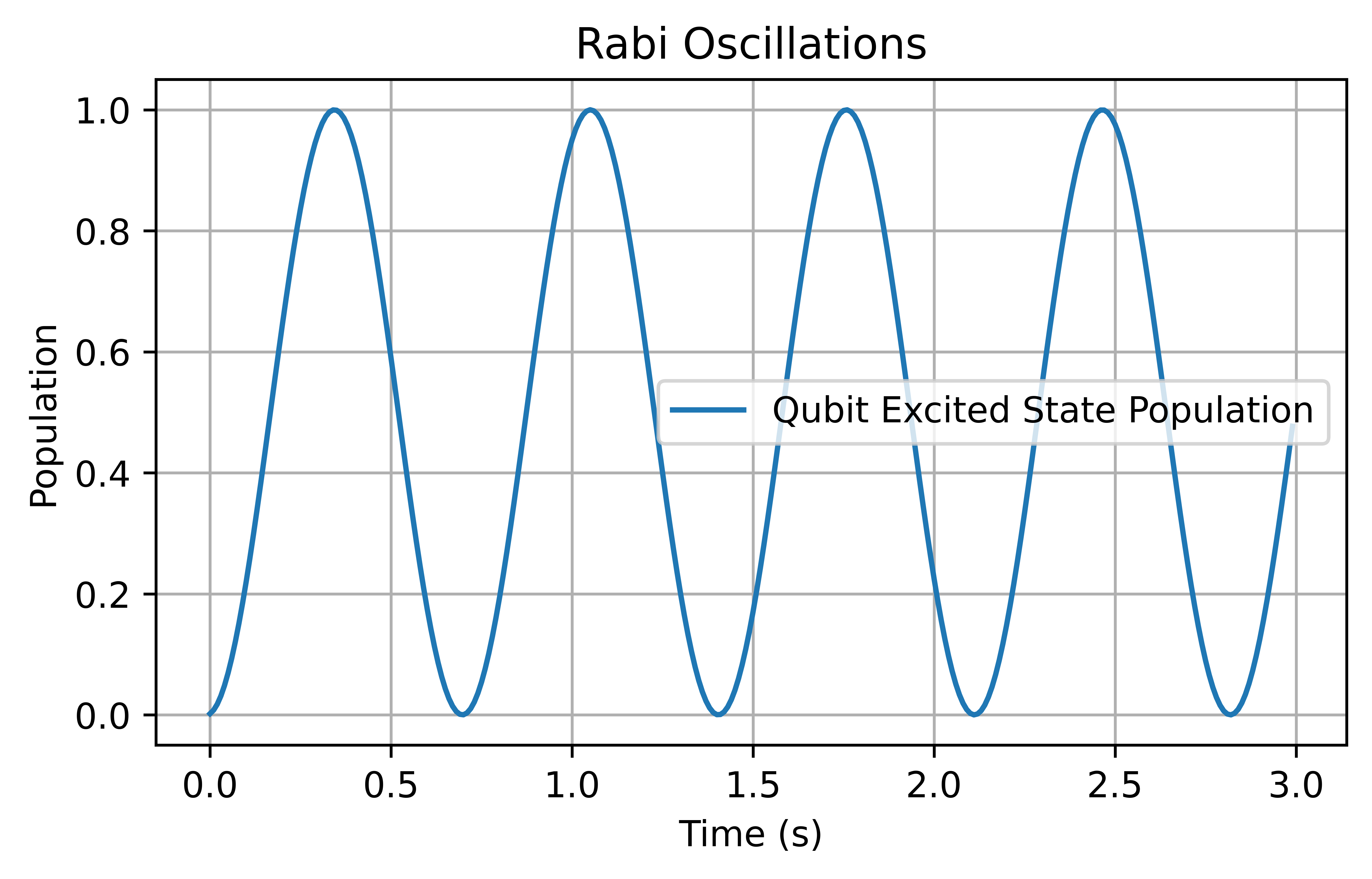
5. Plot the interaction
Using the stored populations we can plot the interactions.
plt.figure(figsize=(6, 3.375))
plt.plot(interractions, qubit_excited_populations, label="Qubit Excited State Population")
plt.xlabel("Time (s)")
plt.ylabel("Population")
plt.legend()
plt.grid()
plt.savefig("plots/jc.png", dpi=1000, bbox_inches="tight")